Detailed Explanation of the Principles and Structure of Barcode Scanner |
Part 17: Signal Processing Theory, Analog-to-Digital Conversion, and Decoding Mathematics |
1. Introduction to Signal Processing in Barcode Scanners |
1.1 What signal Processing Means in This Context |
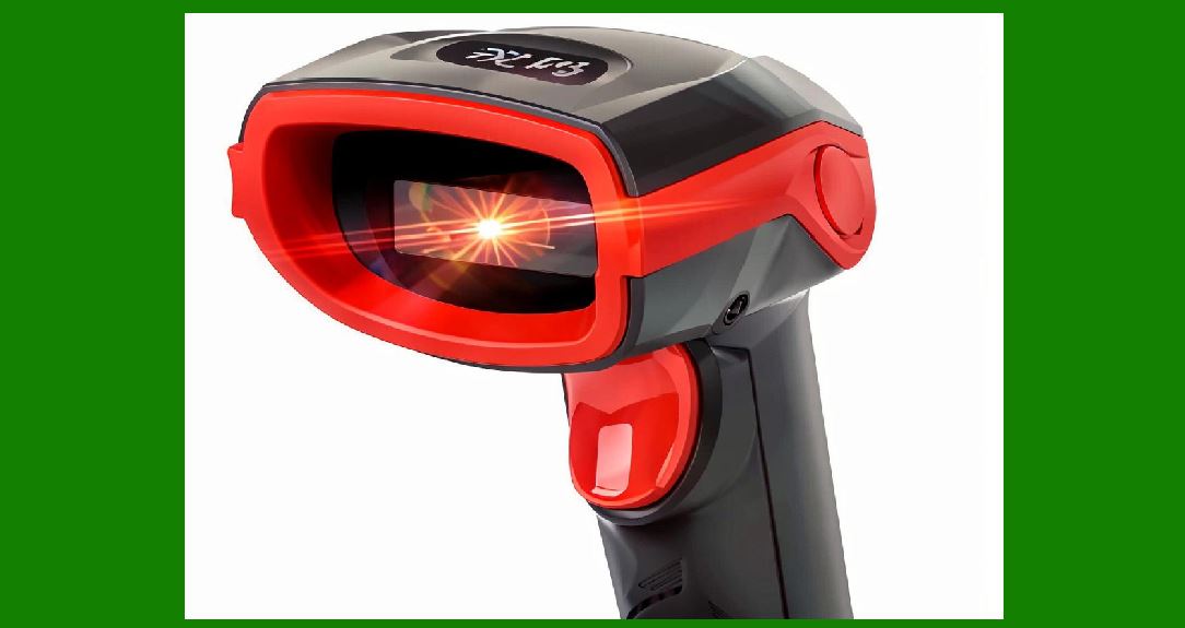
In barcode scanners, signal processing refers to the transformation of raw physical signals (light reflections) into structured digital data that can be decoded. |
This includes: |
1. Converting light into electrical signals |
2. Filtering noise from raw data |
3. Enhancing signal clarity |
4. Extracting meaningful patterns |
5. Preparing data for decoding algorithms |
1.2 Signal Processing Pipeline Overview |
A simplified pipeline is: |
1. Optical reflection (light signal) |
2. Sensor conversion (analog electrical signal) |
3. Amplification and filtering |
4. Analog-to-digital conversion |
5. Digital signal processing |
6. Barcode decoding |
Each stage refines the data further. |
|
2. Analog Signal Generation from Light |
2.1 Light-to-Electrical Conversion |
When light hits a photodiode or CMOS pixel: |
1. Photons generate electron movement |
2. Electrical charge is produced |
3. Signal strength corresponds to brightness |
2.2 Analog Signal Characteristics |
The raw signal is: |
1. Continuous (not digital yet) |
2. Sensitive to noise |
3. Proportional to light intensity |
2.3 Signal Variations from Barcode Structure |
1. Black bars low reflection signal |
2. White spaces high reflection signal |
3. Alternating pattern waveform representation |

|
3. Analog Signal Conditioning |
3.1 Amplification |
Weak signals are strengthened using: |
1. Operational amplifiers |
2. Automatic gain control (AGC) |
Purpose: |
* Improve detectability |
* Normalize signal range |
3.2 Filtering |
Filters remove unwanted components: |
1. Low-pass filters remove high-frequency noise |
2. High-pass filters remove slow drift |
3. Band-pass filters isolate useful frequencies |
3.3 Signal Stabilization |
1. Reduces flicker effects |
2. Smooths irregular variations |
3. Prepares signal for digitization |

|
4. Analog-to-Digital Conversion (ADC) |
4.1 Purpose of ADC |
ADC converts continuous analog signals into discrete digital values. |
4.2 Sampling Process |
1. Signal is sampled at fixed intervals |
2. Each sample is assigned a numeric value |
3. Produces a digital waveform |
4.3 Sampling Rate Importance |
1. Higher sampling rate more accurate representation |
2. Lower sampling rate risk of data loss |
4.4 Quantization |
1. Continuous signal is rounded to discrete levels |
2. Introduces quantization error |
3. Resolution depends on bit depth |
4.5 ADC Bit Depth |
1. 8-bit 256 levels |
2. 10-bit 1024 levels |
3. 12-bit or higher high precision scanning |
|
5. Digital Signal Representation of Barcodes |
5.1 Waveform Conversion |
A barcode becomes a waveform: |
* Peaks = white spaces |
* Valleys = black bars |
5.2 Edge Detection in Signal Form |
1. Rising edge transition from dark to light |
2. Falling edge transition from light to dark |
These edges define barcode structure. |
5.3 Timing Analysis |
1. Width of signals corresponds to encoded data |
2. Timing consistency is critical for decoding |

|
6. Noise in Digital Signals |
6.1 Types of Noise |
1. Thermal noise (sensor-based) |
2. Photon noise (light variability) |
3. Electrical interference |
6.2 Effects of Noise |
1. Distorts signal edges |
2. Causes decoding errors |
3. Reduces accuracy |
6.3 Noise Reduction Techniques |
1. Averaging multiple samples |
2. Digital filtering |
3. Threshold smoothing |
|
7. Signal Thresholding |
7.1 Concept of Thresholding |
Thresholding converts grayscale signal into binary form: |
1. Above threshold white |
2. Below threshold black |
7.2 Adaptive Thresholding |
1. Adjusts based on lighting conditions |
2. Improves performance in uneven illumination |
7.3 Global vs Local Thresholding |
1. Global single threshold for entire image |
2. Local varying thresholds per region |

|
8. Edge Detection Algorithms |
8.1 Purpose |
To identify transitions between bars and spaces. |
8.2 Common Techniques |
1. Gradient-based detection |
2. Sobel operators |
3. Laplacian filters |
8.3 Signal Interpretation |
1. Strong gradient barcode edge |
2. Weak gradient noise or texture |
|
9. Timing-Based Decoding Theory |
9.1 Width Measurement Principle |
Barcode data is encoded in: |
1. Width of bars |
2. Width of spaces |
9.2 Time-Domain Conversion |
1. Scanner converts spatial width into time intervals |
2. Digital processor interprets timing differences |
9.3 Relative Measurement |
1. Absolute size not required |
2. Ratio between elements is sufficient |

|
10. Mathematical Models in Decoding |
10.1 Binary Representation Model |
1. Black = 0 |
2. White = 1 |
3. Sequence forms binary string |
10.2 Pattern Matching Models |
1. Predefined templates |
2. Symbol lookup tables |
10.3 Statistical Decoding |
1. Probability-based interpretation |
2. Error correction weighting |
|
11. Error Detection and Correction Theory |
11.1 Sources of Errors |
1. Noise distortion |
2. Print defects |
3. Motion blur |
11.2 Redundancy in Encoding |
1. Extra bits added for correction |
2. Enables reconstruction of missing data |
11.3 Error Correction Algorithms |
1. Reed-Solomon codes (2D barcodes) |
2. Checksum validation (1D barcodes) |
|
12. Signal Reconstruction |
12.1 Purpose |
To rebuild an ideal barcode signal from noisy input. |
12.2 Techniques |
1. Interpolation of missing data |
2. Curve smoothing |
3. Pattern alignment correction |
|
13. Fourier and Frequency Analysis (Advanced) |
13.1 Frequency Domain View |
Barcode patterns can be analyzed as: |
1. High-frequency transitions (edges) |
2. Low-frequency background variation |
13.2 Fourier Transform Application |
1. Converts signal into frequency components |
2. Helps isolate barcode structure |

|
14. Real-Time Processing Constraints |
14.1 Latency Requirements |
1. Decoding must happen in milliseconds |
2. No noticeable delay for user |
14.2 Stream Processing |
1. Continuous input stream |
2. On-the-fly decoding |

|
15. Hardware-Software Co-Processing |
15.1 Division of Tasks |
1. Hardware signal acquisition |
2. Software interpretation and decoding |
15.2 Acceleration Techniques |
1. DSP offloading |
2. Parallel processing pipelines |

|
16. Future Trends in Signal Processing |
16.1 AI-Based Signal Interpretation |
1. Neural networks decode noisy signals |
2. Adaptive learning from scanning history |
16.2 Fully Digital Optical Chains |
1. Minimal analog processing |
2. Direct digital sensor output |
16.3 Quantum Signal Enhancement (Research Stage) |
1. Ultra-sensitive photon detection |
2. Extreme low-noise environments |

|
17. Summary of Part 17 |
In this section, we explored how raw optical signals are transformed into decoded barcode data: |
1. Light-to-electrical signal conversion |
2. Analog signal conditioning |
3. ADC sampling and quantization |
4. Digital waveform representation |
5. Noise sources and filtering techniques |
6. Thresholding and edge detection |
7. Timing-based decoding theory |
8. Mathematical decoding models |
9. Error detection and correction systems |
10. Signal reconstruction techniques |
11. Frequency-domain analysis |
12. Real-time processing constraints |
13. Hardware-software cooperation |
14. Future AI-driven signal processing trends |
Signal processing is the core bridge between physical barcode patterns and meaningful digital information. |

|
Next Step |
In Part 18, we will explore: |
* Barcode decoding algorithms in detail |
* 1D vs 2D decoding logic structures |
* Pattern recognition and template matching |
* Error correction decoding workflows |
 cs@easiersoft.com