Part 21: High-Speed Imaging Architecture and Frame Rate Optimization in Image-Based Scanners |
1. Introduction to High-Speed Imaging in Scanners |
1. High-speed imaging is a core requirement in modern image-based scanners, especially in retail checkout systems, high-throughput logistics, and industrial automation lines. |
2. The goal is to capture and process images at a speed sufficient to: |
* Track moving objects |
* Reduce motion blur |
* Increase scanning success rate per second |
3. High-speed imaging is not only about camera frame rate it is a full system optimization problem involving: |
* Sensor technology |
* Memory bandwidth |
* Processing pipelines |
* Illumination synchronization |
* Decoding efficiency |

|
2. Imaging Pipeline in High-Speed Mode |
2.1 Core Pipeline Stages |
1. Image exposure |
2. Sensor readout |
3. Frame buffering |
4. ISP processing |
5. Localization and decoding |
6. Output transmission |
2.2 Real-Time Constraints |
1. Each frame must be processed within a strict time budget. |
2. Example constraint model: |
* 60 FPS system ~16.67 ms per frame |
* 120 FPS system ~8.33 ms per frame |

|
3. Image Sensor Technologies for High Speed |
3.1 Rolling Shutter Sensors |
1. Common in low-cost scanners. |
2. Limitation: |
* Distortion during motion capture |
3.2 Global Shutter Sensors |
1. Capture entire frame simultaneously. |
2. Advantages: |
* Eliminates motion skew |
* Critical for high-speed environments |
3.3 High-Speed CMOS Architectures |
1. Features: |
* Parallel pixel readout |
* Column-level ADCs |
* Reduced latency pipelines |

|
4. Frame Rate Optimization Techniques |
4.1 Exposure Time Reduction |
1. Short exposure reduces motion blur. |
2. Trade-off: |
* Lower brightness |
* Increased noise |
4.2 Frame Skipping Strategies |
1. Process only relevant frames. |
2. Used when: |
* Scene is stable |
* Object movement is predictable |
4.3 Adaptive Frame Rate Control |
1. System dynamically adjusts FPS based on: |
* Motion detection |
* Lighting conditions |

|
5. High-Speed Data Transfer Architecture |
5.1 Sensor-to-Processor Bandwidth |
1. High-speed interfaces: |
* MIPI CSI-2 |
* Parallel LVDS (in some designs) |
5.2 Memory Bandwidth Bottleneck |
1. Frames must be stored temporarily in: |
* SRAM |
* DDR memory |
5.3 Double and Triple Buffering |
1. Enables: |
* Continuous capture |
* Parallel processing |
|
6. Processing Acceleration for High Frame Rates |
6.1 Parallel Pipeline Processing |
1. Different frames processed simultaneously at different stages. |
6.2 Hardware Acceleration |
1. Dedicated ISP blocks handle: |
* Filtering |
* Scaling |
* Edge detection |
6.3 SIMD and Vectorization |
1. Pixel-level operations executed in parallel. |

|
7. Illumination Synchronization for High-Speed Imaging |
7.1 Strobe Lighting |
1. LED flashes synchronized with sensor exposure. |
7.2 Duty-Cycled Illumination |
1. Light activated only during capture window. |
7.3 Flicker-Free Illumination Design |
1. Eliminates interference from ambient lighting cycles. |

|
8. Motion Compensation Techniques |
8.1 Motion Detection Algorithms |
1. Detect movement before decoding begins. |
8.2 Frame Stabilization |
1. Align multiple frames to reduce motion blur. |
8.3 Optical Flow Estimation |
1. Tracks pixel movement across frames. |

|
9. High-Speed Decoding Strategies |
9.1 Early ROI Detection |
1. Identify barcode region quickly to avoid full-frame processing. |
9.2 Progressive Decoding |
1. Partial decoding while image is still being processed. |
9.3 Multi-Threaded Decoding Engines |
1. Parallel execution of decoding attempts. |

|
10. Latency Reduction Techniques |
10.1 Pipeline Parallelism |
1. Overlapping capture, processing, and decoding stages. |
10.2 Hardware Offloading |
1. ISP and DSP handle compute-heavy tasks. |
10.3 Zero-Copy Memory Access |
1. Eliminates unnecessary data duplication. |

|
11. Bottlenecks in High-Speed Imaging Systems |
11.1 Sensor Readout Delay |
1. Limited by pixel architecture. |
11.2 Memory Access Contention |
1. Multiple modules competing for bandwidth. |
11.3 Processing Overload |
1. CPU/DSP saturation under high frame rates. |

|
12. Performance Optimization Trade-offs |
12.1 Frame Rate vs Image Quality |
1. Higher FPS: |
* Lower exposure |
* Increased noise |
12.2 Power Consumption vs Speed |
1. Faster processing increases energy usage. |
12.3 Resolution vs Throughput |
1. Higher resolution reduces maximum achievable FPS. |

|
13. Industrial High-Speed Applications |
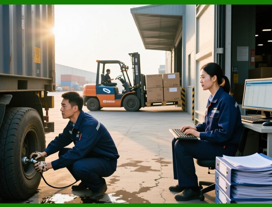
13.1 Conveyor Belt Scanning |
1. Objects moving at high speed require: |
* Global shutter sensors |
* High-intensity strobe lighting |
13.2 Automated Sorting Systems |
1. Multi-object tracking at high frame rates. |
13.3 High-Density Packaging Lines |
1. Rapid scanning of tightly packed items. |
|
14. Emerging High-Speed Imaging Technologies |
14.1 Event-Based Vision Sensors |
1. Capture only changes in scene. |
14.2 Ultra-High Frame Rate Sensors |
1. Hundreds to thousands of FPS for specialized systems. |
14.3 AI-Driven Frame Prediction |
1. Predict missing frames using neural networks. |

|
15. Future Trends in High-Speed Imaging |
15.1 Fully Parallel Imaging Pipelines |
1. Near-zero latency architectures. |
15.2 Sensor-Level AI Processing |
1. Decoding begins inside sensor hardware. |
15.3 Optical Computing Integration |
1. Use of optical signals for preprocessing. |

|
16. Summary of Part 21 |
1. High-speed imaging is a system-wide optimization problem, not just a camera specification. |
2. Global shutter sensors are essential for motion-free capture. |
3. Frame rate optimization requires balancing speed, power, and image quality. |
4. Pipeline parallelism and hardware acceleration are critical. |
5. Future systems will move toward event-based sensors and AI-driven predictive imaging. |

|
Next Step |
Part 22: Embedded Software Architecture and Real-Time Operating System (RTOS) Design in Image-Based Scanners |
 cs@easiersoft.com